
Plus haut, nous avons défini le membre de droite d'un
système de taille \(m\times n\), à savoir ''\(A\boldsymbol{x}\)'', comme le produit d'une matrice
\(A\) de taille \(m\times n\) par le vecteur \(\boldsymbol{x}\in\mathbb{R}^n\).
Ce produit étant défini comme une combinaison linéaire des colonnes de \(A\),
\(A\boldsymbol{x}\) est un vecteur de \(\mathbb{R}^m\).
La multiplication par une matrice de taille \(m\times n\) est donc une opération
qui transforme les vecteurs de \(\mathbb{R}^n\) en des vecteurs
de \(\mathbb{R}^m\). C'est un cas particulier d'une
application (ou fonction) de \(\mathbb{R}^n\) dans \(\mathbb{R}^m\):
\[\begin{aligned}
\mathbb{R}^n&\to \mathbb{R}^m\\
\boldsymbol{x}&\mapsto A\boldsymbol{x}\,.
\end{aligned}\]
Si nécessaire, quelques notions générales sur les fonctions sont rappelées
ici
.
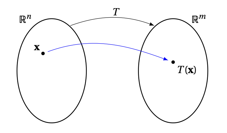
Plus généralement, une application n'est pas forcément définie à l'aide d'une matrice. On utilisera souvent la lettre ''\(T\)'' pour représenter une application générique: \[\begin{aligned} T:\mathbb{R}^n&\to \mathbb{R}^m\\ \boldsymbol{x}&\mapsto T(\boldsymbol{x})\,. \end{aligned}\]
Le vecteur \(\boldsymbol{y}=T(\boldsymbol{x})\) est appelé image de \(\boldsymbol{x}\) (par
\(T\)), et \(\boldsymbol{x}\) est une préimage de \(\boldsymbol{y}\).
Considérons un instant une équation du type suivant
\[ (*)\,:\, T(\boldsymbol{x})=\boldsymbol{b}\,,
\]
où le membre de droite \(\boldsymbol{b}\in\mathbb{R}^m\) est fixé.
L'existence d'au moins une solution \(\boldsymbol{x}\in \mathbb{R}^n\), pour cette équation,
revient à demander si \(\boldsymbol{b}\) fait partie des
éléments de l'ensemble d'arrivée qui sont ''atteints'' par l'application,
c'est-à-dire pour lesquels il existe au moins une préimage. Ceci mène à la
définition suivante:
On a donc, pour l'équation \((*)\) ci-dessus:
Remarque: Si \(T : \mathbb{R}^n \to \mathbb{R}^m\) est une application linéaire, alors \(T(\boldsymbol{0}) = \boldsymbol{0}\). En effet, la définition d'application linéaire nous dit que \[ T(\boldsymbol{0}) = T(\boldsymbol{0} + 1.\boldsymbol{0}) = T(\boldsymbol{0}) + 1.T(\boldsymbol{0}) = T(\boldsymbol{0}) + T(\boldsymbol{0}). \] Si l'on considère la somme du membre initial et du membre final de l'identité précédente avec \(-T(\boldsymbol{0})\), on conclut que \(\boldsymbol{0} = T(\boldsymbol{0})\).
Remarque: On laisse comme exercice la preuve du fait qu'une application \(T : \mathbb{R}^n \to \mathbb{R}^m\) est linéaire si et seulement si elle satisfait aux deux propriétés suivantes:
Exemple: Considérons l'application \(T:\mathbb{R}^3\to \mathbb{R}^2\) définie ainsi: \[ \begin{pmatrix} x_1\\ x_2\\ x_3 \end{pmatrix} =\boldsymbol{x} \mapsto T(\boldsymbol{x}):= \begin{pmatrix} -x_1+3x_2+5x_3\\ x_3+7x_1 \end{pmatrix}\,. \] Montrons, ''à la main'', uniquement à l'aide de la définition de linéarité, que \(T\) est linéaire. Pour ce faire, prenons un \(\boldsymbol{x}= \begin{pmatrix} x_1\\ x_2\\ x_3 \end{pmatrix}\) et un scalaire \(\lambda\). On utilise la définition de \(T\) pour calculer \[\begin{aligned} T(\lambda \boldsymbol{x})&= T\begin{pmatrix} \lambda x_1\\ \lambda x_2\\ \lambda x_3 \end{pmatrix}\\ &= \begin{pmatrix} (-\lambda x_1)+3(\lambda x_2)+5(\lambda x_3)\\ (\lambda x_3)+7(\lambda x_1) \end{pmatrix}\\ &=\lambda \begin{pmatrix} - x_1+3 x_2+5\lambda x_3\\ x_3+7x_1 \end{pmatrix}\\ &=\lambda T(\boldsymbol{x})\,. \end{aligned}\] Ensuite, pour toute paire \(\boldsymbol{x},\boldsymbol{y}\), \[\begin{aligned} T(\boldsymbol{x}+\boldsymbol{y})&= T \begin{pmatrix} x_1+y_1\\ x_2+y_2\\ x_3+y_3 \end{pmatrix} \\ &= \begin{pmatrix} -(x_1+y_1)+3(x_2+y_2)+5(x_3+y_3)\\ (x_3+y_3)+7(x_1+y_1) \end{pmatrix}\\ &= \begin{pmatrix} -x_1+3x_2+5x_3\\ x_3+7x_1 \end{pmatrix}+ \begin{pmatrix} -y_1+3y_2+5y_3\\ y_3+7y_1 \end{pmatrix}\\ &=T(\boldsymbol{x})+T(\boldsymbol{y})\,. \end{aligned}\] On a donc bien montré que \(T\) est linéaire.
Nous avons déjà vu que si \(T:\mathbb{R}^n\to\mathbb{R}^m\), et s'il existe une matrice de taille \(m\times n\) telle que \[ T(\boldsymbol{x})= A\boldsymbol{x}\,\qquad \forall \boldsymbol{x}\in\mathbb{R}^n\,,\] alors \(T\) est linéaire . Mais a priori, une application peut être linéaire sans forcément être associée à une matrice.
Exemple: Si on reprend l'application \(T\) de l'exemple précédent, on peut remarquer que \[ T(\boldsymbol{x})= \begin{pmatrix} -x_1+3x_2+5x_3\\ x_3+7x_1 \end{pmatrix} = \underbrace{ \begin{pmatrix} -1&3&5\\ 7&0&1 \end{pmatrix} }_{=:A} \begin{pmatrix} x_1\\ x_2\\ x_3 \end{pmatrix} =A\boldsymbol{x}\,. \] Ainsi, \(T\) est linéaire.
Pour montrer qu'une application n'est pas linéaire, il suffit de montrer qu'une des deux conditions qui définit la linéarité n'est pas satisfaite, en exhibant un contre-exemple. On pourra donc
Exemple: Considérons l'application \(T:\mathbb{R}^2\to\mathbb{R}^3\) définie par \[ \begin{pmatrix} x_1\\x_2 \end{pmatrix}=\boldsymbol{x} \mapsto T(\boldsymbol{x}):= \begin{pmatrix} x_1x_2\\ -x_2\\ x_1 \end{pmatrix}\,. \] L'apparition de la multiplication ''\(x_1x_2\)'' indique que cette application n'est probablement pas linéaire. Comme contre-exemple, prenons \(\lambda=2\), et \(\boldsymbol{x}_*= \begin{pmatrix} 1\\3 \end{pmatrix} \). On a \[ T(\lambda\boldsymbol{x}_*) =T\left( 2 \begin{pmatrix} 1\\3 \end{pmatrix} \right) =T \begin{pmatrix} 2\\6 \end{pmatrix} = \begin{pmatrix} 12\\ -6\\ 2 \end{pmatrix}\,, \] alors que \[ \lambda T(\boldsymbol{x}_*)=2T \begin{pmatrix} 1\\3 \end{pmatrix} =2 \begin{pmatrix} 3\\ -3\\ 1 \end{pmatrix} = \begin{pmatrix} 6\\ -6\\ 2 \end{pmatrix}\,. \] On a donc \(T(\lambda\boldsymbol{x}_*)\neq \lambda T(\boldsymbol{x}_*)\), ce qui implique que \(T\) n'est pas linéaire.
Point clé: Équivalence entre SEL et applications linéaires
Résoudre un SEL
\[
(*)
\left\{
\begin{array}{ccccccccc}
a_{1,1}x_1&+&a_{1,2}x_2&+&\cdots&+&a_{1,n}x_n&=&b_1\,,\\
a_{2,1}x_1&+&a_{2,2}x_2&+&\cdots&+&a_{2,n}x_n&=&b_2\,,\\
\vdots&&&&&&&\vdots&\\
a_{m,1}x_1&+&a_{m,2}x_2&+&\cdots&+&a_{m,n}x_n&=&b_m\,,
\end{array}
\right. \,
\]
est équivalent à
trouver toutes les préimages de
\(\boldsymbol{b} \in \mathbb{R}^m\)
par l'application linéaire
\(T:\mathbb{R}^n \rightarrow \mathbb{R}^m \)
donnée par \(T(\boldsymbol{x})=A\boldsymbol{x}\) pour \(\boldsymbol{x} \in \mathbb{R}^n\),
où \(A\) est la matrice du SEL \( (*) \) et \(\boldsymbol{b}\) est le vecteur formé du
second membre du \( (*) \).
Dernière compilation: 2025-09-02 (09:33:29)
Sauf indication contraire, le contenu de ce document est soumis à une licence Creative Commons internationale, Attribution: Pas d'Utilisation Commerciale - Partage dans les Mêmes Conditions 4.0 (CC BY-NC-SA 4.0)
