6.8 Formule de Cramer et conséquences\({}^{{\color{red}\star}}\)
Résolution de systèmes d'équations linéaires par déterminants
Dans cette sous-section, on présente une application intéressante de
la théorie du déterminant à la résolution des systèmes linéaires.
Si \(A\) est une matrice inversible de taille
\(n\times n\), on sait que pour tout \(\boldsymbol{b}\in
\mathbb{R}^n\), le système
\[ A\boldsymbol{x}=\boldsymbol{b}
\]
possède exactement une solution \(\boldsymbol{x}\), donnée par
\[
\boldsymbol{x}=A^{-1}\boldsymbol{b}\,.
\]
Nous allons voir comment il est possible de calculer chacune des composantes
\(x_j\) de cette solution, sans passer par la connaissance de \(A^{-1}\).
Si \(M\) est une matrice de taille \(n\times n\), et \(\boldsymbol{z}\in \mathbb{R}^n\),
\(M_j(\boldsymbol{z})\) est la matrice de taille \(n\times n\) obtenue à partir de \(M\)
en remplaçant la \(j\)-ème colonne par \(\boldsymbol{z}\) (sans toucher aux autres
colonnes).
Exemple:
Si \(M= \begin{pmatrix} 1&2&3\\ 4&5&6\\ 7&8&9 \end{pmatrix} \),
\(\boldsymbol{z}= \begin{pmatrix} \sqrt{2}\\\pi\\e \end{pmatrix} \), alors
\[
M_2(\boldsymbol{z})=
\begin{pmatrix}
1&\sqrt{2}&3\\
4&\pi&6\\
7&e&9
\end{pmatrix}
\,.\]
(Formule de Cramer)
Soit \(A\) une matrice de taille \(n\times n\) inversible, \(\boldsymbol{b}\in \mathbb{R}^n\), et
soit \(\boldsymbol{x}\in\mathbb{R}^n\) l'unique solution du système \(A\boldsymbol{x}=\boldsymbol{b}\).
Alors pour tout \(j\in\{1,2,\dots,n\}\), la \(j\)-ème composante de \(\boldsymbol{x}\)
est égale à
\[
x_j=\frac{\det\big(A_j(\boldsymbol{b})\big)}{\det(A)}\,.
\]
Exemple:
Considérons le système linéaire \(A\boldsymbol{x}=\boldsymbol{b}\) donné par
\[
(*)\quad
\begin{pmatrix}
1&2&3&4\\
1&2&3&0\\
1&2&0&0\\
1&0&0&0
\end{pmatrix}
\begin{pmatrix} x_1\\ x_2\\ x_3\\ x_4 \end{pmatrix}
=
\begin{pmatrix} 5\\ 6\\ 7\\ 8 \end{pmatrix}\,.
\]
Comme \(\det(A)=4!=24\neq 0\), la matrice est inversible et la solution du système est
unique. Si on s'intéresse par exemple à la quatrième composante \(x_4\),
\[\begin{aligned}
x_4=\frac{\det\big(A_4(\boldsymbol{b})\big)}{\det(A)}
&=\frac{1}{24}\det
\begin{pmatrix}
1&2&3&5\\
1&2&3&6\\
1&2&0&7\\
1&0&0&8
\end{pmatrix}\\
&=\frac{1}{4}\det
\begin{pmatrix}
1&1&1&5\\
1&1&1&6\\
1&1&0&7\\
1&0&0&8
\end{pmatrix}\\
&=\frac{1}{4}\det
\begin{pmatrix}
0&0&1&5\\
0&0&1&6\\
0&1&0&7\\
1&0&0&8
\end{pmatrix}\,.
\end{aligned}\]
On a d'abord
extrait un \(2\) de la deuxième colonne et un \(3\) de la troisième, puis on a
soustrait la deuxième colonne de la première, et la troisième de la deuxième.
Maintenant, en développant selon la première colonne,
\[\begin{aligned}
x_4&=\frac{1}{4}\det
\begin{pmatrix}
0&0&1&5\\
0&0&1&6\\
0&1&0&7\\
1&0&0&8
\end{pmatrix}\\
&=\frac{1}{4}(-1)\det
\begin{pmatrix}
0&1&5\\
0&1&6\\
1&0&7\\
\end{pmatrix}\\
&=\frac{1}{4}(-1)(1)\det
\begin{pmatrix}
1&5\\
1&6\\
\end{pmatrix}\\
&=\frac{1}{4}(-1)(1)(6-5)\\
&=-\frac{1}{4}\,.
\end{aligned}\]
Bien-sûr, on trouve la même chose qu'en résolvant
complètement le système \((*)\), qui serait par exemple de faire
\(L_1\leftarrow L_1-L_2\),
\(L_2\leftarrow L_2-L_3\),
\(L_3\leftarrow L_3-L_4\), qui donne
\[
\begin{pmatrix}
0&0&0&4\\
0&0&3&0\\
0&2&0&0\\
1&0&0&0
\end{pmatrix}
\begin{pmatrix} x_1\\ x_2\\ x_3\\ x_4 \end{pmatrix}
=
\begin{pmatrix} -1\\ -1\\ -1\\ 8 \end{pmatrix}\,.
\]
Une application intéressante: formule pour \(A^{-1}\)
Si le système considéré est grand, la
formule de Cramer pour \(x_j\)
représente un intérêt limité du point de vue calculatoire. En effet elle
implique le calcul de deux déterminants, qui comme on sait représente un nombre
d'opérations croissant factoriellement avec la taille du système.
Par contre, d'un point de vue théorique elle permet de dériver une formule
explicite pour l'inverse d'une matrice:
Soit \(A\) une matrice de taille \(n\times n\) inversible.
La matrice complémentaire de \(A\) est la matrice \( \operatorname{Comp}(A) \) de taille \(n\times n\) dont les coefficients sont donnés par
\[
\operatorname{Comp}(A)_{i,j}
:= (-1)^{i+j} \det(A[j|i])
\]
pour tout \(1 \leqslant i,j \leqslant n\).
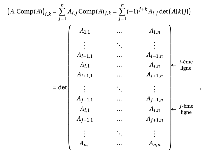
Théorème:
Soit \(A\) une matrice de taille \(n\times n\).
Alors
\[
A.\operatorname{Comp}(A) = \operatorname{Comp}(A). A = \det(A) I_n.
\]
En conséquence, si \(A\) est inversible,
l'inverse de \(A\) est donnée par
\[ A^{-1}=\frac{1}{\det(A)}\operatorname{Comp}(A)\,.
\]
Exemple:
La matrice
\[A=
\begin{pmatrix}
2&1&3\\
1&-1&1\\
1&4&-2
\end{pmatrix}\,,
\]
est inversible puisque \(\det(A)=-14\neq 0\).
Utilisons la formule pour calculer son inverse. Indiquons
en rouge le signe de chaque coefficient, venant du
\((-1)^{i+j}={\color{red}\pm 1}\) dans la
matrice complémentaire.
\[\begin{aligned}
A^{-1}
=& \frac{1}{\det(A)}\operatorname{Comp}(A)\\
=\frac{1}{-14}&
\begin{pmatrix}
{\color{red}+}\det
\begin{pmatrix} -1&1\\ 4&-2 \end{pmatrix}
&
{\color{red}-}\det
\begin{pmatrix} 1&3\\ 4&-2 \end{pmatrix}
&
{\color{red}+}\det
\begin{pmatrix} 1&3\\ -1&1 \end{pmatrix}
\\
{\color{red}-}\det
\begin{pmatrix} 1&1\\ 1&-2 \end{pmatrix}
&{\color{red}+}\det
\begin{pmatrix} 2&3\\ 1&-2 \end{pmatrix}
&
{\color{red}-}\det
\begin{pmatrix} 2&3\\ 1&1 \end{pmatrix}
\\
{\color{red}+}\det
\begin{pmatrix} 1&-1\\ 1&4 \end{pmatrix}
&{\color{red}-}\det
\begin{pmatrix} 2&1\\ 1&4 \end{pmatrix}
&{\color{red}+}\det
\begin{pmatrix} 2&1\\ 1&-1 \end{pmatrix}
\end{pmatrix}\\
&=\frac{1}{-14}
\begin{pmatrix}
-2&14&4\\
3 14&-7&1\\
5&-7&-3
\end{pmatrix}\,.
\end{aligned}\]