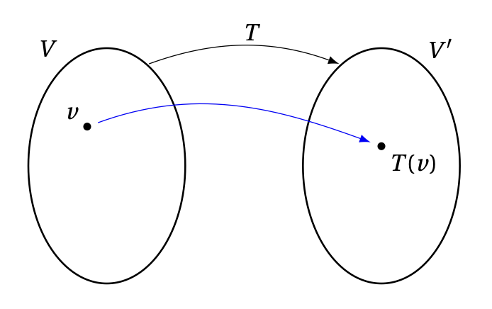
Considérons deux espaces vectoriels, \(V\) et \(V'\), ainsi qu'une application linéaire \(T:V\to V'\).
Supposons maintenant que ces deux espaces vectoriels sont tous deux de dimension finie, chacun muni d'une base:
Nous allons voir maintenant comment l'utilisation de ces bases va permettre de ramener l'étude de \(T\) à l'étude d'une application linéaire de \(\mathbb{R}^p\) dans \(\mathbb{R}^m\).
Théorème: Soient \(V\) et \(V'\) deux espaces vectoriels, avec des bases \(\mathcal{B}\) et \(\mathcal{B}'\), respectivement. On suppose que \(\dim (V) = n\) et \(\dim (V') = m\). Soit \(T : V \rightarrow V' \) une application linéaire. Alors, \[ \big[T(v)\big]_{\mathcal{B}'} = [T]_{\mathcal{B}'\leftarrow\mathcal{B}} [v]_{\mathcal{B}} \] pour tout \(v \in V\). En plus, \([T]_{\mathcal{B}'\leftarrow\mathcal{B}}\) est l'unique matrice qui satisfait \eqref{eq:mat-app-lin}, i.e. si \(A\) est une matrice de taille \(m \times n\) telle que \([T(v)]_{\mathcal{B}'} = A [v]_{\mathcal{B}}\) pour tout \(v \in V\), alors \( A = [T]_{\mathcal{B}'\leftarrow\mathcal{B}}\).
Étant donne \(v\in V\), décomposons-le sur \(\mathcal{B}\): \[v=a_1v_1+\dots+a_pv_p\,,\] ce qui permet de décrire \(v\) univoquement à l'aide du vecteur de \(\mathbb{R}^p\) qui lui est associé: \[ [v]_\mathcal{B} = \begin{pmatrix} a_1\\ \vdots\\ a_p \end{pmatrix} \,. \] Ensuite, regardons l'image de \(v\) par \(T\). Puisque \(T\) est linéaire, \[\begin{aligned} T(v) &=T(a_1v_1+\dots+a_pv_p)\\ &=a_1T(v_1)+\dots+a_pT(v_p)\,. \end{aligned}\] En utilisant ensuite la linéarité de \([\cdot]_{\mathcal{B}'}\), \[\begin{aligned} \big[T(v)\big]_{\mathcal{B}'} &=\big[a_1T(v_1)+\dots+a_pT(v_p)\big]_{\mathcal{B}'}\\ &=a_1\big[T(v_1)\big]_{\mathcal{B}'}+\dots+a_p\big[T(v_p)\big]_{\mathcal{B}'}\,. \end{aligned}\] Cette dernière ligne est une combinaison linéaire des vecteurs \([T(v_1)]_{\mathcal{B}'},\cdots,[T(v_p)]_{\mathcal{B}'}\) de \(\mathbb{R}^m\), on peut donc l'interpréter comme un produit d'une matrice par le vecteur \([v]_{\mathcal{B}}\): \[\begin{aligned} \big[T(v)\big]_{\mathcal{B}'} = a_1\big[T(v_1)\big]_{\mathcal{B}'}+\dots+a_p\big[T(v_p)\big]_{\mathcal{B}'} &= \underbrace{\Bigl[\big[T(v_1)\big]_{\mathcal{B}'} \cdots \big[T(v_p)\big]_{\mathcal{B}'}\Big]}_{m\times n} \underbrace{\begin{pmatrix} a_1\\ \vdots\\ a_p \end{pmatrix}}_{=[v]_{\mathcal{B}}}\\ &= \Big[\big[T(v_1)\big]_{\mathcal{B}'} \cdots \big[T(v_p)\big]_{\mathcal{B}'}\Big] [v]_\mathcal{B}\,, \end{aligned}\] comme on voulait démontrer. Finalement, pour montrer l'unicité, il suffit de noter que \(A[v_i]_{\mathcal{B}} = A\boldsymbol{e}_i\) est la \(i\)-ème colonne de \(A\) pour tout \(1\leqslant i \leqslant n\).
Ce que nous avons fait ci-dessus peut se résumer dans le shéma suivant:
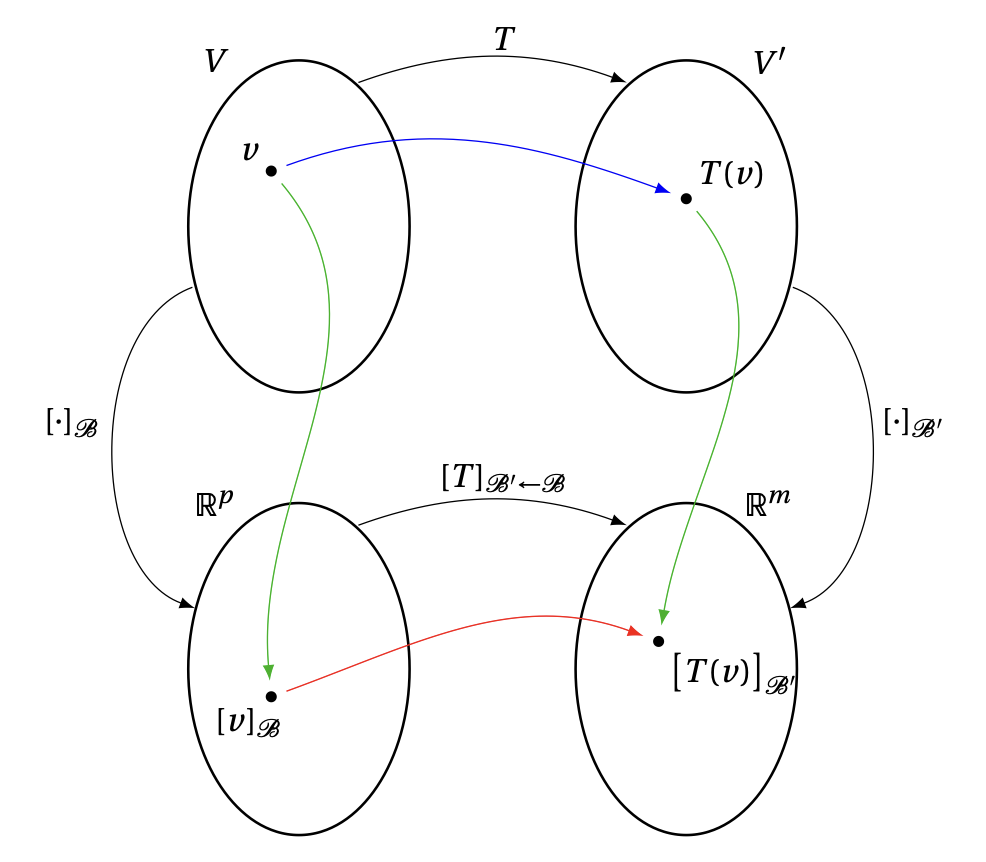
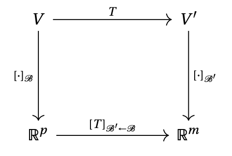
En utilisant les bases \(\mathcal{B}\) et \(\mathcal{B}'\), ainsi que les applications \([\cdot]_{\mathcal{B}}\) et \([\cdot]_{\mathcal{B}'}\) qui leur sont associées, nous avons pu prendre l'application \[{\color{blue}v\mapsto T(v)}\,\] qui est abstraite, et nous l'avons rendue plus concrète, en la représentant à l'aide d'une matrice: on peut maintenant la voir comme une application linéaire de \(\mathbb{R}^p\) dans \(\mathbb{R}^m\), dont la matrice est \([T]_{\mathcal{B}'\mathcal{B}}\): \[ \underbrace{{\color{red}[v]_\mathcal{B}}}_{\in \mathbb{R}^p} \,\, {\color{red}\mapsto} \,\, \underbrace{{\color{red}\big[T(v)\big]_{\mathcal{B}'}}}_{\in \mathbb{R}^m} = {\color{red} [T]_{\mathcal{B}'\leftarrow\mathcal{B}} [v]_\mathcal{B} }\,. \] En conséquence, l'étude de \(T\) peut se réduire à celle de la matrice \([T]_{\mathcal{B}'\leftarrow\mathcal{B}}\).
Point clé: Matrice d'une application linéaire et vecteurs de coordonnées
Pour une application linéaire \(T : V \rightarrow V' \), et bases \(\mathcal{B}\) de \(V\) et \(\mathcal{B}'\) de \(V'\), on a l'identité
fondamentale
\begin{equation*}
\(\big[T(v)\big]_{\mathcal{B}'}
=
[T]_{\mathcal{B}'\leftarrow\mathcal{B}}
[v]_{\mathcal{B}}\)
\end{equation*}
pour tout \(v \in V\), et
\([T]_{\mathcal{B}'\leftarrow\mathcal{B}}\) est
l'unique matrice qui vérifie cette propriété pour tout \(v \in V\).
Exemple:
Considérons l'application \(T:\mathbb{P}_3\to \mathbb{P}_2\) définie ainsi:
pour \(p\in \mathbb{P}_3\),
\[
T(p)=p'\,,
\]
i.e. \(T(p)(t):= p'(t)\) pour tout \( t \in \mathbb{R} \),
où \(p'(t)\) est la dérivée de \(p\) par rapport à \(t\).
Cette application est clairement linéaire puisque
\[
T(\alpha p+\beta q)=(\alpha p+\beta q)'=\alpha p'+\beta q'=
\alpha T(p)+\beta T(q)\,.
\]
Calculons maintenant la matrice associée à cette application relative
Exemple: Considérons l'application \[\begin{aligned} T:\mathbb{P}_2&\to\mathbb{R}^2\\ p&\mapsto T(p):= \begin{pmatrix} p(0)\\p'(1) \\ \end{pmatrix}\,, \end{aligned}\] où \(p'(t)\) désigne la dérivée de \(p(t)\) par rapport à \(t\). Remarquons que \(T\) est linéaire, puisque pour tous \(p,q\in \mathbb{P}_2\) et tout scalaires \(\alpha,\beta\), \[\begin{aligned} T(\alpha p+\beta q) &= \begin{pmatrix} \alpha p(0)+\beta q(0)\\ \alpha p'(1)+\beta q'(1) \end{pmatrix}\\ &= \alpha \begin{pmatrix} p(0)\\ p'(1) \end{pmatrix} + \beta \begin{pmatrix} q(0)\\ q'(1) \end{pmatrix} =\alpha T(p)+\beta T(q)\,. \end{aligned}\] Puisqu'on connaît la base canonique \(\mathcal{B}_{\mathrm{can}}=\{e_0,e_1,e_2\}\) dans \(\mathbb{P}_2\) et la base canonique \(\mathcal{B}_{\mathrm{can}}'=\{\boldsymbol{e}_1,\boldsymbol{e}_2\}\) dans \(\mathbb{R}^2\) (on écrit \(\mathcal{B}_{\mathrm{can}}'\) juste pour la distinguer de l'autre, mais c'est bien la base canonique de \(\mathbb{R}^2\)), on peut calculer la matrice de taille \(2\times 3\) qui représente \(T\) relative à ces bases: \[ [T]_{\mathcal{B}_{\mathrm{can}}'\leftarrow\mathcal{B}_{\mathrm{can}}} = \Big[\big[T(e_0)\big]_{\mathcal{B}_{\mathrm{can}}'}\,\big[T(e_1)\big]_{\mathcal{B}_{\mathrm{can}}'}\,\big[T(e_2)\big]_{\mathcal{B}_{\mathrm{can}}'}\Big]\,. \] Comme \(e_0(t)=1\), \(e_1(t)=t\), \(e_2(t)=t^2\), on a \[\begin{aligned} T(e_0)&= \begin{pmatrix} e_0(0)\\ e_0'(1) \end{pmatrix} = \begin{pmatrix} 1\\ 0 \end{pmatrix}\,,\\ T(e_1)&= \begin{pmatrix} e_1(0)\\ e_1'(1) \end{pmatrix} = \begin{pmatrix} 0\\ 1\end{pmatrix}\,,\\ T(e_2)&= \begin{pmatrix} e_2(0)\\ e_2'(1) \end{pmatrix} = \begin{pmatrix} 0\\ 2\end{pmatrix}\,, \end{aligned}\] et donc \[ [T]_{\mathcal{B}_{\mathrm{can}}'\leftarrow\mathcal{B}_{\mathrm{can}}} = \begin{pmatrix} 1&0&0\\ 0&1&2 \end{pmatrix}\,. \] Par exemple, prenons le polynôme \(p(t)=9-2t+7t^2\), et calculons son image. Alors \[\begin{aligned} \big[T(p)\big]_{\mathcal{B}_{\mathrm{can}}'} &= [T]_{\mathcal{B}_{\mathrm{can}}'\leftarrow\mathcal{B}_{\mathrm{can}}}[p]_{\mathcal{B}_{\mathrm{can}}}\\ &= \begin{pmatrix} 1&0&0\\ 0&1&2 \end{pmatrix} \begin{pmatrix} 9\\ -2\\ 7 \end{pmatrix} = \begin{pmatrix} 9\\12 \end{pmatrix}\,, \end{aligned}\] qui est bien \( \begin{pmatrix} p(0)\\p'(1) \end{pmatrix} \).
On présente les propriétés fondamentales des représentations matricielles des applications linéaires.
On montre d'abord la première identité. Pour le faire, étant donné \(v \in V\), on a \[ [S \circ T]_{\mathcal{B}'' \leftarrow \mathcal{B}} [v]_{\mathcal{B}} = \big[(S\circ T)(v)\big]_{\mathcal{B}''} = \Big[S\big(T(v)\big)\Big]_{\mathcal{B}''} = [S]_{\mathcal{B}'' \leftarrow \mathcal{B}'}\big[T(v)\big]_{\mathcal{B}'} = [S]_{\mathcal{B}'' \leftarrow \mathcal{B}'} [T]_{\mathcal{B}' \leftarrow \mathcal{B}} [v]_{\mathcal{B}}\,. \] Par l'unicité de la représentation matricielle dans le théorème %(cliquer) précédent, on conclut que \( [S \circ T]_{\mathcal{B}'' \leftarrow \mathcal{B}} = [S]_{\mathcal{B}'' \leftarrow \mathcal{B}'} [T]_{\mathcal{B}' \leftarrow \mathcal{B}}\). Pour montrer la deuxième identité, noter que \[ I_{\dim(V)}[v]_{\mathcal{B}} = [v]_{\mathcal{B}} = \big[\mathrm{id}_V(v)\big]_{\mathcal{B}} = [\mathrm{id}_V]_{\mathcal{B} \leftarrow \mathcal{B}} [v]_{\mathcal{B}} \] pour tout \(v \in V\). L'unicité de la représentation matricielle dans le théorème %(cliquer) précédent nous dit que \( [\mathrm{id}_V]_{\mathcal{B} \leftarrow \mathcal{B}} = I_{\dim(V)}\). On prouve maintenant l'item \hyperlink{(INJ-r)} {(INJ)}. On suppose que \(\dim(V) = n\) et \(\dim(V') = m\). Alors, \[\begin{aligned} v \in \mathrm{Ker}(T) &\Leftrightarrow T(v) = \mathbf{0}_{V'} \Leftrightarrow \big[T(v)\big]_{\mathcal{B}'} = \mathbf{0} \\ &\Leftrightarrow [T]_{\mathcal{B}'\leftarrow\mathcal{B}} [v]_{\mathcal{B}} = \mathbf{0} \Leftrightarrow [v]_{\mathcal{B}} \in \mathrm{Ker}\big([T]_{\mathcal{B}' \leftarrow \mathcal{B}}\big)\,, \end{aligned}\] où l'on a utilisé dans la deuxième équivalence que \([\cdot]_{\mathcal{B}'} : V' \rightarrow \mathbb{R}^m\) est bijective, et dans dans la troisième équivalence l'identité fondamentale \[ \big[T(v)\big]_{\mathcal{B}'} = [T]_{\mathcal{B}'\leftarrow\mathcal{B}} [v]_{\mathcal{B}} \] pour \(v \in V\). La dernière partie de l'item \hyperlink{(INJ-r)} {(INJ)} suit du fait qu'une application linéaire est injective si et seulement si son noyau est réduit à zéro (voir le dernier Lemme %(cliquer) dans la Section (cliquer)). On montre l'item \hyperlink{(SUR-r)} {(SUR)}. On suppose que \(\dim(V) = n\) et \(\dim(V') = m\). Alors, \[\begin{aligned} v' \in \mathrm{Im} (T) &\Leftrightarrow \text{il existe } v \in V \text{ tel que }T(v) = v' \Leftrightarrow \text{il existe } v \in V \text{ tel que } \big[T(v)\big]_{\mathcal{B}'} = [v']_{\mathcal{B}'} \\ &\Leftrightarrow \text{il existe } v \in V \text{ tel que } [T]_{\mathcal{B}'\leftarrow\mathcal{B}} [v]_{\mathcal{B}} = [v']_{\mathcal{B}'} \\ &\Leftrightarrow \text{il existe } \boldsymbol{x} \in \mathbb{R}^n \text{ tel que } [T]_{\mathcal{B}'\leftarrow\mathcal{B}} \boldsymbol{x} = [v']_{\mathcal{B}'} \Leftrightarrow [v']_{\mathcal{B}'} \in \mathrm{Im} \big([T]_{\mathcal{B}' \leftarrow \mathcal{B}}\big)\,, \end{aligned}\] où l'on a utilisé dans la deuxième équivalence que \([\cdot]_{\mathcal{B}'} : V' \rightarrow \mathbb{R}^m\) est bijective, dans la troisième équivalence l'identité fondamentale \[ \big[T(v)\big]_{\mathcal{B}'} = [T]_{\mathcal{B}'\leftarrow\mathcal{B}} [v]_{\mathcal{B}} \] pour \(v \in V\), et dans la quatrième équivalence que \([\cdot]_{\mathcal{B}} : V \rightarrow \mathbb{R}^n\) est bijective. La dernière partie de l'item \hyperlink{(SUR-r)} {(SUR)} suit directement de ce que l'on a montré précédemment et du fait que \([\cdot]_{\mathcal{B}} : V' \rightarrow \mathbb{R}^m\) est bijective. On va finalement prouver l'item \hyperlink{(INV-r)} {(INV)}. On suppose que \(T\) est bijective et on montrera que \([T]_{\mathcal{B}' \leftarrow \mathcal{B}}\) est inversible et \([T]_{\mathcal{B}' \leftarrow \mathcal{B}}^{-1} =[T^{-1}]_{\mathcal{B} \leftarrow \mathcal{B}'}\). Comme \(T\) est bijective, soit \(T^{-1}\) l'application réciproque. Alors, les deux premiers items nous disent que \[ I_{\dim(V)} = [\mathrm{id}_V]_{\mathcal{B} \leftarrow \mathcal{B}} = [T^{-1} \circ T]_{\mathcal{B} \leftarrow \mathcal{B}} = [T^{-1}]_{\mathcal{B} \leftarrow \mathcal{B}'} [T]_{\mathcal{B}' \leftarrow \mathcal{B}} \] et \[ I_{\dim(V')} = [\mathrm{id}_{V'}]_{\mathcal{B}' \leftarrow \mathcal{B}'} = [T \circ T^{-1}]_{\mathcal{B}' \leftarrow \mathcal{B}'} = [T]_{\mathcal{B}' \leftarrow \mathcal{B}} [T^{-1}]_{\mathcal{B} \leftarrow \mathcal{B}'}\,. \] En conséquence, \([T]_{\mathcal{B}' \leftarrow \mathcal{B}}\) est inversible et \([T]_{\mathcal{B}' \leftarrow \mathcal{B}}^{-1} =[T^{-1}]_{\mathcal{B} \leftarrow \mathcal{B}'}\). Réciproquement, si \([T]_{\mathcal{B}' \leftarrow \mathcal{B}}\) est une matrice inversible, alors elle est injective et surjective, et, d'après les items \hyperlink{(INJ-r)} {(INJ)} et \hyperlink{(SUR-r)} {(SUR)}, \(T\) est injective et surjective, i.e. bijective, comme on voulait démontrer.
Nous reviendrons plus en profondeur sur la représentation d'une application linéaire à l'aide d'une matrice, en particulier dans le cas \(T:\mathbb{R}^n\to\mathbb{R}^m\).
Dernière compilation: 2025-09-02 (09:33:30)
Sauf indication contraire, le contenu de ce document est soumis à une licence Creative Commons internationale, Attribution: Pas d'Utilisation Commerciale - Partage dans les Mêmes Conditions 4.0 (CC BY-NC-SA 4.0)
