8.4 Les matrices de passage
Motivation
Pour commencer, étudions les relations existant entre les composantes d'un
même vecteur, exprimé relativement à une base ou à une autre.
Avant de voir l'approche dans le cas général,
commençons par un exemple simple.
Exemple:
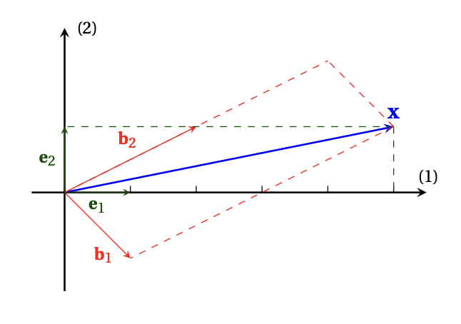
Dans le plan, considérons le vecteur
\[
\boldsymbol{x}= \begin{pmatrix} 5\\ 1 \end{pmatrix}\,.
\]
Considérons maintenant la base \(\mathcal{B}=\{ \boldsymbol{b}_1,\boldsymbol{b}_2 \}\), dont les
vecteurs sont disons
\[
\boldsymbol{b}_1= \begin{pmatrix} 1\\-1 \end{pmatrix}\,,\qquad
\boldsymbol{b}_2= \begin{pmatrix} 2\\1 \end{pmatrix}\,.
\]
Quelles sont les composantes de \(\boldsymbol{x}\) relatives à \(\mathcal{B}\)?
Ce qu'on cherche ici est
\[ [\boldsymbol{x}]_\mathcal{B}=
\begin{pmatrix}\beta_1 \\\beta_2 \end{pmatrix}\,,
\]
qui ne signifie rien d'autre que
\[ \boldsymbol{x}=\beta_1\boldsymbol{b}_1+\beta_2\boldsymbol{b}_2\,.
\]
Or cette dernière s'exprime comme
\[
\begin{pmatrix} 5\\1 \end{pmatrix}
=
\beta_1
\begin{pmatrix} 1\\-1 \end{pmatrix}
+\beta_2
\begin{pmatrix} 2\\1 \end{pmatrix}\,,
\]
qui est équivalent au système d'équations linéaires
\[
\left\{
\begin{array}{ccccc}
\beta_1 &+& 2\beta_2 &=& 5\,,
\\
-\beta_1 &+& \beta_2 &=&1\,,
\end{array}
\right.
\]
dont la solution est \(\beta_1=1\), \(\beta_2=2\).
Ainsi,
\[ [\boldsymbol{x}]_\mathcal{B}=
\begin{pmatrix}1 \\2 \end{pmatrix}\,,
\]
qui signifie \(\boldsymbol{x}=\boldsymbol{b}_1+2\boldsymbol{b}_2\).
Remarque: Il est plus utile de penser que \(\boldsymbol{x}\) est un vecteur dans
le plan, et que ce vecteur peut être représenté en composantes, relatives à
la base canonique \(\mathcal{B}_{\mathrm{can}}\) ou à la base \(\mathcal{B}\):
\[
[\boldsymbol{x}]_{\mathcal{B}_{\mathrm{can}}}=
\begin{pmatrix}5 \\1 \end{pmatrix}\,,
\qquad
[\boldsymbol{x}]_\mathcal{B}=
\begin{pmatrix}1 \\2 \end{pmatrix}\,.
\]
Bien-sûr, il serait intéressant d'avoir un procédé permettant d'obtenir
directement les composantes d'un vecteur quelconque dans une base, en fonction
des composantes dans l'autre base:
\[
[\boldsymbol{x}]_{\mathcal{B}_{\mathrm{can}}}=
\begin{pmatrix}\gamma_1 \\\gamma_2 \end{pmatrix}
\overset{?}{\longleftrightarrow}
\begin{pmatrix}\beta_1 \\\beta_2 \end{pmatrix}
=[\boldsymbol{x}]_\mathcal{B}\,.
\]
Abordons le problème d'un point de vue général.
Soit \(V\) un espace vectoriel de dimension \(p\).
Supposons que l'on ait deux bases dans \(V\):
\[
\mathcal{B}=\{ b_1,\dots,b_p\}\,,\qquad \mathcal{C}=\{c_1,\dots,c_p\}\,.
\]
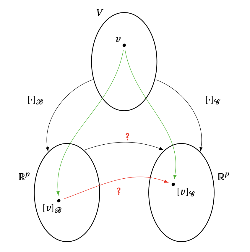
Si \(v\in V\) est un vecteur quelconque, il peut être décomposé dans une base ou
dans l'autre, et les composantes relatives à ces bases seront a priori
différentes:
\[
[v]_\mathcal{B}=
\begin{pmatrix}
\beta_1\\
\vdots\\
\beta_p
\end{pmatrix}\,,
\qquad
[v]_\mathcal{C}=
\begin{pmatrix}
\gamma_1\\
\vdots\\
\gamma_p
\end{pmatrix}\,.
\]
Nous aimerions savoir comment les composantes relatives à
une base, par exemple les
\(\beta_1,\dots,\beta_p\), peuvent se calculer à partir des composantes dans
l'autre base, c'est-à-dire les \(\gamma_1,\dots,\gamma_p\).
Le but de la prochaine sous-section c'est de voir que cette relation est linéaire, et peut donc s'exprimer à
l'aide d'une matrice.
La définition de matrice de passage
On rappelle l'application identité
\(\mathrm{id}_V :V\to V\), définie par
\[
\mathrm{id}_V(v):= v\,,\qquad \forall v\in V\,.
\]
Cette application ne porte en elle rien de vraiment intéressant.
Mais considérons comme avant deux bases pour décrire \(V\), notées
\(\mathcal{C}\) et \(\mathcal{B}\).
Soit \(V\) un espace vectoriel de dimension finie et soient \(\mathcal{B}\) et \(\mathcal{C}\) deux bases de \(V\).
La matrice de passage (ou de changement de base) de \(\mathcal{B}\) vers \(\mathcal{C}\), notée \(P_{\mathcal{C}\leftarrow\mathcal{B}}\), est définie via
\[
P_{\mathcal{C}\leftarrow\mathcal{B}} := [\mathrm{id}_V]_{\mathcal{C}\leftarrow\mathcal{B}}.
\]
Étant un cas particulier de représentation matricielle d'une application linéaire,
on trouve immédiatement plusieurs propriétés des matrices de passage.
Soit \(V\) un espace vectoriel de dimension finie et soient \(\mathcal{B} =\{b_1, \dots,b_p\}\) et \(\mathcal{C} = \{ c_1, \dots, c_p\) deux bases de \(V\).
Alors,
- \(P_{\mathcal{C}\leftarrow\mathcal{B}}=\bigl[[b_1]_\mathcal{C}\cdots [b_p]_\mathcal{C}\bigr]\),
- \([v]_{\mathcal{C}}=P_{\mathcal{C}\leftarrow\mathcal{B}}[v]_{\mathcal{B}}\) pour tout \(v \in V\);
- \(P_{\mathcal{C}\leftarrow\mathcal{B}}\) est inversible et
\({P_{\mathcal{C}\leftarrow\mathcal{B}}}^{-1}=P_{\mathcal{B}\leftarrow\mathcal{C}}\).
Preuve:
Le premier item suit de la définition de représentation matricielle, vu que
\[
P_{\mathcal{C}\leftarrow\mathcal{B}}
=
[\mathrm{id}_V]_{\mathcal{C}\leftarrow\mathcal{B}}
=\Big[\big[\mathrm{id}_V(b_1)\big]_{\mathcal{C}} \cdots
\big[\mathrm{id}_V(b_p)\big]_{\mathcal{C}} \Big]
=
\bigl[[b_1]_\mathcal{C}\cdots [b_p]_\mathcal{C}\bigr]\,.
\]
Le deuxième item suit de l'identité
du Théorème
dans la Section (cliquer)
pour \(T = \mathrm{id}_V\).
Finalement, comme l'application \(\mathrm{id}_V\) est bijective, le dernier item
de la Proposition
dans la Section (cliquer)
nous dit que \(P_{\mathcal{C}\leftarrow\mathcal{B}} = [\mathrm{id}_V]_{\mathcal{C}\leftarrow\mathcal{B}}\) est inversible.
En plus, la même proposition nous dit que
\[
P_{\mathcal{C}\leftarrow\mathcal{B}}^{-1} = [\mathrm{id}_V]_{\mathcal{C}\leftarrow\mathcal{B}}^{-1}
= [\mathrm{id}_V^{-1}]_{\mathcal{B}\leftarrow\mathcal{C}}
= [\mathrm{id}_V]_{\mathcal{B}\leftarrow\mathcal{C}}
= P_{\mathcal{B}\leftarrow\mathcal{C}}
\,,
\]
où l'on a utilisé dans la dernière égalité que \(\mathrm{id}_V^{-1} = \mathrm{id}_V\).
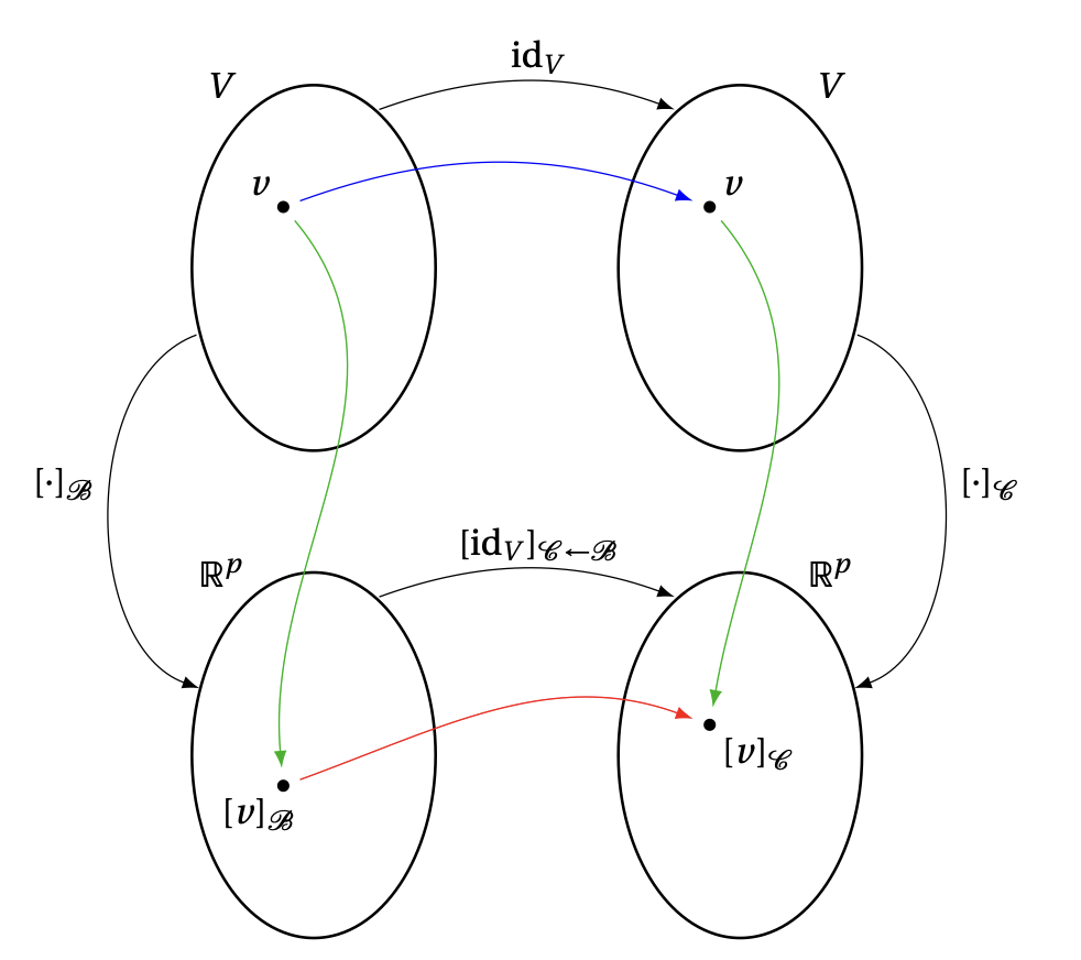
On peut représenter la matrice de passage de forme graphique via le diagramme suivant.
On présente aussi de façon sommaire le point clé de cette section.
Point clé: Matrice de passage et vecteurs de coordonnées
Pour un espace vectoriel \(V\) de dimension finie, et bases \(\mathcal{B}\) et
\(\mathcal{C}\) de \(V\), on a l'identité fondamentale
\begin{equation*}
\([v]_{\mathcal{C}}
=
P_{\mathcal{C}\leftarrow\mathcal{B}}
[v]_{\mathcal{B}}\)
\end{equation*}
pour tout \(v \in V\), et \(P_{\mathcal{C}\leftarrow\mathcal{B}}\) est l'unique matrice qui
vérifie cette propriété pour tout \(v \in V\).
Exemple:
Dans le plan, considérons comme tout à l'heure le vecteur
\[
\boldsymbol{x}= \begin{pmatrix} 5\\ 1 \end{pmatrix}\,.
\]
Pour être plus précis, notons \(\mathcal{B}_{\mathrm{can}}=\{\boldsymbol{e}_1,\boldsymbol{e}_2\}\) la base canonique,
et récrivons
\[
[\boldsymbol{x}]_{\mathcal{B}_{\mathrm{can}}}= \begin{pmatrix} 5\\ 1 \end{pmatrix}\,.
\]
Considérons maintenant la base \(\mathcal{B}=\{\boldsymbol{b}_1,\boldsymbol{b}_2\}\) définie par:
\[
\boldsymbol{b}_1= \begin{pmatrix} 1\\-1 \end{pmatrix}\,,\qquad
\boldsymbol{b}_2= \begin{pmatrix} 2\\1 \end{pmatrix}\,.
\]
Calculons \([\boldsymbol{x}]_\mathcal{B}\), en fonction de
\([\boldsymbol{x}]_{\mathcal{B}_{\mathrm{can}}}\), en utilisant le théorème:
\[
[
\boldsymbol{x}]_\mathcal{B} =P_{\mathcal{B}\leftarrow\mathcal{B}_{\mathrm{can}}} [\boldsymbol{x}]_{\mathcal{B}_{\mathrm{can}}} \,,
\]
où
\[P_{\mathcal{B}\leftarrow\mathcal{B}_{\mathrm{can}}}=\bigl[[\boldsymbol{e}_1]_\mathcal{B}\,[\boldsymbol{e}_2]_\mathcal{B}\bigr]\,.\]
On doit donc
trouver les composantes de \(\boldsymbol{e}_1\) et \(\boldsymbol{e}_2\) relatives
à \(\mathcal{B}\).
Mais comme
\[
[\boldsymbol{b}_1]_{\mathcal{B}_{\mathrm{can}}}=\begin{pmatrix} 1\\-1 \end{pmatrix}\,,\qquad
[\boldsymbol{b}_2]_{\mathcal{B}_{\mathrm{can}}}=\begin{pmatrix} 2\\1 \end{pmatrix}\,
\]
signifie en fait
\[
\left\{
\begin{array}{ccccc}
\boldsymbol{b}_1&=&\boldsymbol{e}_1&-&\boldsymbol{e}_2\,, \\
\boldsymbol{b}_2&=&2\boldsymbol{e}_1&+&\boldsymbol{e}_2 \,,
\end{array}
\right.
\]
on a
\[
\left\{
\begin{array}{ccccc}
\boldsymbol{e}_1&=&\frac13\boldsymbol{b}_1&+&\frac13\boldsymbol{b}_2\,, \\
\boldsymbol{e}_2&=&-\frac23\boldsymbol{b}_1&+&\frac13\boldsymbol{b}_2 \,,
\end{array}
\right.
\]
Ainsi,
\[
[\boldsymbol{e}_1]_\mathcal{B}= \begin{pmatrix} 1/3\\ 1/3 \end{pmatrix} \,,\qquad
[\boldsymbol{e}_2]_\mathcal{B}= \begin{pmatrix} -2/3\\ 1/3 \end{pmatrix} \,,
\]
et donc
\[
P_{\mathcal{B}\leftarrow\mathcal{B}_{\mathrm{can}}}=\bigl[[\boldsymbol{e}_1]_\mathcal{B}\,[\boldsymbol{e}_2]_\mathcal{B}\bigr]
=
\begin{pmatrix}
1/3&-2/3\\
1/3&1/3
\end{pmatrix}\,.
\]
Donc les coordonnées de \(\boldsymbol{x}\) relatives à \(\mathcal{B}\) sont
\[
[\boldsymbol{x}]_\mathcal{B}=P_{\mathcal{B}\leftarrow\mathcal{B}_{\mathrm{can}}}[\boldsymbol{x}]_{\mathcal{B}_{\mathrm{can}}}=
\begin{pmatrix}
1/3&-2/3\\
1/3&1/3
\end{pmatrix}
\begin{pmatrix} 5\\1 \end{pmatrix}
=
\begin{pmatrix} 1\\2 \end{pmatrix}\,,
\]
comme nous avions trouvé plus haut.
Si maintenant on souhaite plutôt transformer des
composantes relatives à \(\mathcal{B}\) en des composantes relatives à
\(\mathcal{B}_{\mathrm{can}}\), on calcule
\[
P_{\mathcal{B}_{\mathrm{can}}\leftarrow\mathcal{B}}={P_{\mathcal{B}\leftarrow\mathcal{B}_{\mathrm{can}}}}^{-1}
=
\frac{1}{1/3}
\begin{pmatrix} 1/3&2/3\\ -1/3&1/3 \end{pmatrix}
=
\begin{pmatrix} 1&2\\ -1&1 \end{pmatrix}\,.
\]
Donc si par exemple on prend \(\boldsymbol{x}\) tel que
\[
[\boldsymbol{x}]_\mathcal{B}=
\begin{pmatrix} 1\\ 2 \end{pmatrix}\,,
\]
alors ses composantes relatives à \(\mathcal{B}_{\mathrm{can}}\) sont, comme on sait déjà,
\[
[\boldsymbol{x}]_{\mathcal{B}_{\mathrm{can}}}
= P_{\mathcal{B}_{\mathrm{can}}\leftarrow\mathcal{B}}[\boldsymbol{x}]_\mathcal{B}
=
\begin{pmatrix} 1&2\\ -1&1 \end{pmatrix}
\begin{pmatrix} 1\\ 2 \end{pmatrix}
=\begin{pmatrix} 5\\ 1 \end{pmatrix}\,.
\]
Exemple:
Supposons que l'on considère, dans \(\mathbb{R}^3\), le vecteur
\[ \boldsymbol{x}= \begin{pmatrix} 1\\ 2\\ 3 \end{pmatrix}\,. \]
Considérons la base de \(\mathbb{R}^3\), \(\mathcal{B}=\{\boldsymbol{b}_1,\boldsymbol{b}_2,\boldsymbol{b}_3\}\),
dont les vecteurs sont
(on laisse au lecteur le soin de vérifier que \(\mathcal{B}\) est effectivement une
base):
\[
\boldsymbol{b}_1= \begin{pmatrix} 0\\ 0\\ 1 \end{pmatrix}\,,\qquad
\boldsymbol{b}_2= \begin{pmatrix} 1\\ 0\\ -1 \end{pmatrix}\,,\qquad
\boldsymbol{b}_3= \begin{pmatrix} 0\\ 2\\ 0 \end{pmatrix}\,.
\]
Ensuite, cherchons les composantes de \(\boldsymbol{x}\)
relatives à \(\mathcal{B}\), en utilisant le formalisme présenté plus haut.
Pour bien faire, récrivons explicitement ce que nous savons:
\[ [\boldsymbol{x}]_{\mathcal{B}_{\mathrm{can}}}= \begin{pmatrix} 1\\ 2\\ 3 \end{pmatrix}\,, \]
ainsi que
\[
[\boldsymbol{b}_1]_{\mathcal{B}_{\mathrm{can}}}= \begin{pmatrix} 0\\ 0\\ 1 \end{pmatrix}\,,\qquad
[\boldsymbol{b}_2]_{\mathcal{B}_{\mathrm{can}}}= \begin{pmatrix} 1\\ 0\\ -1 \end{pmatrix}\,,\qquad
[\boldsymbol{b}_3]_{\mathcal{B}_{\mathrm{can}}}= \begin{pmatrix} 0\\ 2\\ 0 \end{pmatrix}\,.
\]
Pour exprimer les composantes de \(\boldsymbol{x}\)
relatives à \(\mathcal{B}\), nous allons utiliser la formule
\[
[\boldsymbol{x}]_\mathcal{B}=P_{\mathcal{B}\leftarrow\mathcal{B}_{\mathrm{can}}}[\boldsymbol{x}]_{\mathcal{B}_{\mathrm{can}}}\,,
\]
où la matrice de passage est donnée par
\[ P_{\mathcal{B}\leftarrow\mathcal{B}_{\mathrm{can}}}=
\bigl[
[\boldsymbol{e}_1]_{\mathcal{B}}\, [\boldsymbol{e}_1]_{\mathcal{B}}\, [\boldsymbol{e}_1]_{\mathcal{B}} \bigr]\,.
\]
Or si on écrit explicitement les définitions des vecteurs de la base \(\mathcal{B}\),
\[
\left\{
\begin{array}{ccccc}
\boldsymbol{b}_1 &=&&& \boldsymbol{e}_3\,,\\
\boldsymbol{b}_2 &=&\boldsymbol{e}_1&&-\boldsymbol{e}_3\,, \\
\boldsymbol{b}_3 &=&&2\boldsymbol{e}_2\,.&
\end{array}
\right.
\]
Comme on doit exprimer les composantes des vecteurs de la base canonique par
rapport à \(\mathcal{B}\), il faut inverser ces relations. On trouve facilement
\[
\left\{
\begin{array}{ccccc}
\boldsymbol{e}_1 &=&\boldsymbol{b}_1&+\boldsymbol{b_2}\,,&\\
\boldsymbol{e}_2 &=&&&\frac12 \boldsymbol{b}_3\,, \\
\boldsymbol{e}_3 &=&\boldsymbol{b}_1\,,&&
\end{array}
\right.
\]
c'est-à-dire
\[
[\boldsymbol{e}_1]_{\mathcal{B}}= \begin{pmatrix}1 \\1 \\0 \end{pmatrix}\,,\qquad
[\boldsymbol{e}_2]_{\mathcal{B}}= \begin{pmatrix}0 \\0 \\ \frac12 \end{pmatrix}\,,\qquad
[\boldsymbol{e}_3]_{\mathcal{B}}= \begin{pmatrix}1 \\0 \\0 \end{pmatrix}\,,
\]
ce qui donne
\[\begin{aligned}
[\boldsymbol{x}]_\mathcal{B}
&=P_{\mathcal{B}\leftarrow\mathcal{B}_{\mathrm{can}}}[\boldsymbol{x}]_{\mathcal{B}_{\mathrm{can}}}\\
&=
\begin{pmatrix}
1&0&1\\
1&0&0\\
0&\frac12&0
\end{pmatrix}
\begin{pmatrix} 1\\ 2\\ 3 \end{pmatrix}\\
&=
\begin{pmatrix} 4\\ 1\\ 1 \end{pmatrix}\,.
\end{aligned}\]
Remarque:
Pour le calcul de \(P_{\mathcal{B}\leftarrow\mathcal{B}_{\mathrm{can}}}\), une façon tout à fait
équivalente de faire mais écrite différemment
aurait été de commencer par calculer
\[
P_{\mathcal{B}_{\mathrm{can}}\leftarrow\mathcal{B}}=
\bigl[
[\boldsymbol{b}_1]_{\mathcal{B}_{\mathrm{can}}}\, [\boldsymbol{b}_2]_{\mathcal{B}_{\mathrm{can}}}\, [\boldsymbol{b}_3]_{\mathcal{B}_{\mathrm{can}}} \bigr]
=
\begin{pmatrix}
0&1&0\\
0&0&2\\
1&-1&0
\end{pmatrix}\,,
\]
puis de calculer son inverse (par exemple avec l'algorithme de Gauss-Jordan):
\[
P_{\mathcal{B}\leftarrow\mathcal{B}_{\mathrm{can}}}=
{P_{\mathcal{B}_{\mathrm{can}}\leftarrow\mathcal{B}}}^{-1}=
\begin{pmatrix}
1&0&1\\
1&0&0\\
0&\frac12&0
\end{pmatrix}\,.
\]