Plus haut, nous avons défini le membre de droite d'un
système \(m\times n\), à savoir ''\(A\boldsymbol{x}\)'', comme le produit d'une matrice
(de taille \(m\times n\)) \(A\) par le vecteur \(\boldsymbol{x}\in\mathbb{R}^n\).
Ce produit étant défini comme une combinaison linéaire des colonnes de \(A\),
\(A\boldsymbol{x}\) est un vecteur de \(\mathbb{R}^m\).
La multiplication par une matrice \(m\times n\) est donc une opération
qui transforme les vecteurs de \(\mathbb{R}^n\) en des vecteurs
de \(\mathbb{R}^m\). C'est un cas particulier d'une
application (ou fonction) de \(\mathbb{R}^n\) dans \(\mathbb{R}^m\):
\[\begin{aligned}
\mathbb{R}^n&\to \mathbb{R}^m\\
\boldsymbol{x}&\mapsto A\boldsymbol{x}\,.
\end{aligned}\]
Si nécessaire, quelques notions générales sur les fonctions sont rappelées
ici.
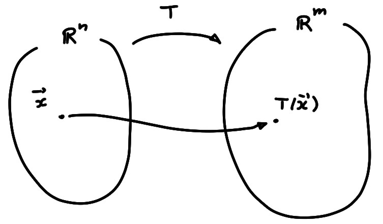
Plus généralement, une application n'est pas forcément définie à l'aide d'une matrice. On utilisera souvent la lettre ''\(T\)'' pour représenter une application générique: \[\begin{aligned} T:\mathbb{R}^n&\to \mathbb{R}^m\\ \boldsymbol{x}&\mapsto T(\boldsymbol{x})\,. \end{aligned}\]
Le vecteur \(\boldsymbol{y}=T(\boldsymbol{x})\) est appelé image de \(\boldsymbol{x}\) (par
\(T\)), et \(\boldsymbol{x}\) est une préimage de \(\boldsymbol{y}\).
Considérons un instant une équation du type suivant
\[ (*)\,:\, T(\boldsymbol{x})=\boldsymbol{b}\,,
\]
où le membre de droite \(\boldsymbol{b}\in\mathbb{R}^m\) est fixé.
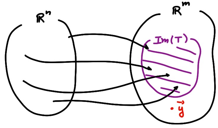
L'existence d'au moins une solution \(\boldsymbol{x}\in \mathbb{R}^n\), pour cette équation,
revient à demander si \(\boldsymbol{b}\) fait partie des
éléments de l'ensemble d'arrivée qui sont ''atteints'' par l'application,
c'est-à-dire pour lesquels il existe au moins une préimage. Ceci mène à la
définition suivante:
On a donc, pour l'équation \((*)\) ci-dessus:
Exemple: Considérons l'application \(T:\mathbb{R}^3\to \mathbb{R}^2\) définie ainsi: \[ \begin{pmatrix} x_1\\ x_2\\ x_3 \end{pmatrix} =\boldsymbol{x} \mapsto T(\boldsymbol{x}):= \begin{pmatrix} -x_1+3x_2+5x_3\\ x_3+7x_1 \end{pmatrix} \] Montrons, ''à la main'', uniquement à l'aide de la définition de linéarité, que \(T\) est linéaire. Pour ce faire, prenons un \(\boldsymbol{x}= \begin{pmatrix} x_1\\ x_2\\ x_3 \end{pmatrix}\) et un scalaire \(\lambda\). On utilise la définition de \(T\) pour calculer \[\begin{aligned} T(\lambda \boldsymbol{x})&= T\Bigl( \begin{pmatrix} \lambda x_1\\ \lambda x_2\\ x_3 \end{pmatrix}\Bigr)\\ &= \begin{pmatrix} (-\lambda x_1)+3(\lambda x_2)+5(\lambda x_3)\\ (\lambda x_3)+7(\lambda x_1) \end{pmatrix}\\ &=\lambda \begin{pmatrix} - x_1+3 x_2+5\lambda x_3\\ x_3+7x_1 \end{pmatrix}\\ &=\lambda T(\boldsymbol{x})\,. \end{aligned}\] Ensuite, pour toute paire \(\boldsymbol{x},\boldsymbol{y}\), \[\begin{aligned} T(\boldsymbol{x}+\boldsymbol{y})&= T\Bigl( \begin{pmatrix} x_1+y_1\\ x_2+y_2\\ x_3+y_3 \end{pmatrix} \Bigr)\\ &= \begin{pmatrix} -(x_1+y_1)+3(x_2+y_2)+5(x_3+y_3)\\ (x_3+y_3)+7(x_1+y_1) \end{pmatrix}\\ &= \begin{pmatrix} -x_1+3x_2+5x_3\\ x_3+7x_1 \end{pmatrix}+ \begin{pmatrix} -y_1+3y_2+5y_3\\ y_3+7y_1 \end{pmatrix}\\ &=T(\boldsymbol{x})+T(\boldsymbol{y})\,. \end{aligned}\] On a donc bien montré que \(T\) est linéaire.
Nous avons déjà vu que si \(T:\mathbb{R}^n\to\mathbb{R}^m\), et si il existe une matrice \(m\times n\) telle que \[ T(\boldsymbol{x})= A\boldsymbol{x}\,\qquad \forall \boldsymbol{x}\in\mathbb{R}^n\,,\] alors \(T\) est linéaire . Mais a priori, une application peut être linéaire sans forcément être associée à une matrice.
Exemple: Si on reprend l'application \(T\) de l'exemple précédent, on peut remarquer que \[ T(\boldsymbol{x})= \begin{pmatrix} -x_1+3x_2+5x_3\\ x_3+7x_1 \end{pmatrix} = \underbrace{ \begin{pmatrix} -1&3&5\\ 7&0&1 \end{pmatrix} }_{=:A} \begin{pmatrix} x_1\\ x_2\\ x_3 \end{pmatrix} =A\boldsymbol{x}\,. \] Ainsi, \(T\) est linéaire.
Pour montrer qu'une application n'est pas linéaire, il suffit de montrer qu'une des deux conditions qui définit la linéarité n'est pas satisfaite, en exhibant un contre-exemple. On pourra donc
Exemple: Considérons l'application \(T:\mathbb{R}^2\to\mathbb{R}^3\) définie par \[ \begin{pmatrix} x_1\\x_2 \end{pmatrix}=\boldsymbol{x} \mapsto T(\boldsymbol{x}):= \begin{pmatrix} x_1x_2\\ -x_2\\ x_1 \end{pmatrix} \] L'apparition de la multiplication ''\(x_1x_2\)'' indique que cette application n'est probablement pas linéaire. Comme contre-exemple, prenons \(\lambda=2\), et \(\boldsymbol{x}_*= \begin{pmatrix} 1\\3 \end{pmatrix} \). On a \[ T(\lambda\boldsymbol{x}_*) =T\Bigl( 2 \begin{pmatrix} 1\\3 \end{pmatrix} \Bigr) =T\Bigl( \begin{pmatrix} 2\\6 \end{pmatrix} \Bigr) = \begin{pmatrix} 12\\ -6\\ 2 \end{pmatrix}\,, \] alors que \[ \lambda T(\boldsymbol{x}_*)=2T\Bigl( \begin{pmatrix} 1\\3 \end{pmatrix} \Bigr) =2 \begin{pmatrix} 3\\ -3\\ 1 \end{pmatrix} = \begin{pmatrix} 6\\ -6\\ 2 \end{pmatrix}\,. \] On a donc \(T(\lambda\boldsymbol{x}_*)\neq \lambda T(\boldsymbol{x}_*)\), ce qui implique que \(T\) n'est pas linéaire.
Nous aurons encore beaucoup à dire sur les
applications linéaires, qui sont les vraies
''fonctions'' étudiées en algèbre linéaire
(un peu comme les fonctions continues sont les fonctions les plus étudiées en
analyse).
Mais avant d'en dire plus, nous allons faire un pause, dans le chapitre suivant,
et reprendre tout ce que nous avons fait jusqu'ici, en adoptant un point de vue
beaucoup plus général, celui des espaces vectoriels abstraits.
Nous introduirons plus de choses dans ce cadre, en particulier à propos des
applications linéaires d'un espace vectoriel dans un autre. Plus tard, nous
appliquerons alors ces notions lorsque nous reviendrons plus en profondeur sur
les applications linéaires du type \(\boldsymbol{x}\mapsto T(\boldsymbol{x})=A\boldsymbol{x}\).
Dernière compilation: 2025-03-16 (08:47:52)
Sauf indication contraire, le contenu de ce document est soumis à une licence Creative Commons internationale, Attribution: Pas d'Utilisation Commerciale - Partage dans les Mêmes Conditions 4.0 (CC BY-NC-SA 4.0)
