8.5 Le changement de base
JE METS CA OU?
On l'a dit, une base permet de représenter les vecteurs d'un espace vectoriel,
de façon univoque.
Pour l'instant, nous avons toujours considéré les vecteurs de
\(\mathbb{R}^n\) comme étant définis à l'aide de leurs composantes relativement à la
base canonique. Cela signifie que lorsqu'on dit qu'un vecteur \(\boldsymbol{x}\) a pour
composantes \(x_1,x_2,\dots, x_n\), cela veut en fait dire que
\[
\boldsymbol{x}=x_1\boldsymbol{e}_1+\cdots +x_n\boldsymbol{e}_n\,.
\]
Donc au lieu de
\[
\boldsymbol{x}=
\begin{pmatrix} x_1\\ \vdots\\ x_n \end{pmatrix}\,,
\]
nous aurions toujours dû écrire
\[
[\boldsymbol{x}]_{\mathcal{B}_{\mathrm{can}}}=
\begin{pmatrix} x_1\\ \vdots\\ x_n \end{pmatrix}\,.
\]
Nous l'avons déjà dit plus haut: les vecteurs existent indépendamment des
composantes que l'on utilise pour les décrire!
Nous allons commencer par exploiter les diverses formules de changement de base
vues dans le chapitre sur les espaces vectoriels, sur quelques exemples
concrets. Nous verrons aussi comment certains problèmes sont plus faciles à
étudier lorsqu'on se place dans une base particulière bien choisie.
Changement de bases: vecteurs
Changement de base pour une application linéaire
Toutes les applications linéaires que nous avons défini jusqu'à présent ont
généralement été définies relativement à la base canonique: leur matrice
s'obtenait en calculant les images des vecteurs de la base canonique.
Mais on sait maintenant exprimer la matrice d'une application relativement à
n'importe quelle base. Nous allons donc repasser par certaines applications
rencontrées précédemment, et étudier leur matrice relativement à des basees qui
ne sont pas canoniques.
Un truc bateau d'une application de \(\mathbb{R}^3\), sans aucun intérêt
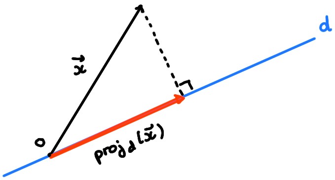
Considérons la projection \(\mathrm{proj}_d\)
sur une droite \(d\) passant par l'origine et faisant
un angle de \(\theta\) avec \(\boldsymbol{e}_1\):
Nous avions trouvé la matrice suivante relativement à la base canonique:
\[
[\mathrm{proj}_d]_{\mathcal{B}_{can}}
=
\begin{pmatrix}
\cos^2\theta&\cos\theta\sin\theta\\
\cos\theta\sin\theta&\sin^2\theta
\end{pmatrix}
\]
L'allure un peu compliquée de cette matrice est due
au fait que l'on a exprimé cette matrice relativement à une base qui n'est pas
naturelle: relativement à \(\mathcal{B}_{\mathrm{can}}=(\boldsymbol{e}_1,\boldsymbol{e}_2)\), \(d\) est inclinée.
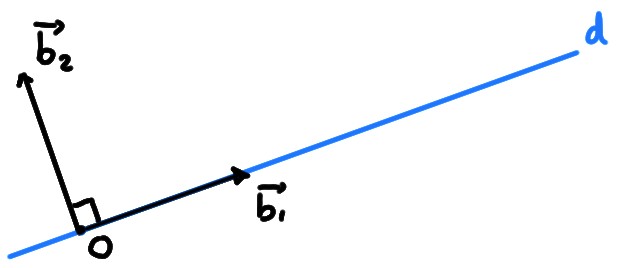
Plus naturelle, pour décrire cette projection, serait une
base dans laquelle les vecteurs sont orientés dans des directions qui tiennent
compte de la position de l'axe \(d\). Par exemple, une base
\(\mathcal{B}=(\boldsymbol{b}_1,\boldsymbol{b}_2)\) où \(\boldsymbol{b}_1\) dirige \(d\), et \(\boldsymbol{b}_2\)
est perpendiculaire à \(d\):
Puisque \(d\) fait un angle \(\theta\) avec l'horizontale, en les prenant
orientés comme sur la figure ci-dessus, et unitaires,
\[
[\boldsymbol{b}_1]_{\mathcal{B}_{\mathrm{can}}}= \begin{pmatrix} \cos\theta\\ \sin\theta \end{pmatrix}\,,\qquad
[\boldsymbol{b}_2]_{\mathcal{B}_{\mathrm{can}}}= \begin{pmatrix} -\sin\theta\\ \cos\theta
\end{pmatrix}\,.
\]
Ainsi, la matrice de changement de base est
\[
P_{\mathcal{B}_{\mathrm{can}}\mathcal{B}}=
\begin{pmatrix}
\cos\theta&-\sin\theta \\
\sin\theta & \cos\theta
\end{pmatrix}\,,
\]
que l'on va utiliser dans la formule de changement de base:
\[
[\mathrm{proj}_d]_{\mathcal{B}}
=
{P_{\mathcal{B}_{\mathrm{can}}\mathcal{B}}}^{-1}
[\mathrm{proj}_d]_{\mathcal{B}_{\mathrm{can}}}
P_{\mathcal{B}_{\mathrm{can}}\mathcal{B}}\,.
\]
On trouve
\[\begin{aligned}
[\mathrm{proj}_d&]_{\mathcal{B}}\\
&=
\begin{pmatrix}
\cos\theta&\sin\theta \\
-\sin\theta & \cos\theta
\end{pmatrix}
\begin{pmatrix}
\cos^2\theta&\cos\theta\sin\theta\\
\cos\theta\sin\theta&\sin^2\theta
\end{pmatrix}
\begin{pmatrix}
\cos\theta&-\sin\theta \\
\sin\theta & \cos\theta
\end{pmatrix}\\
&=
\begin{pmatrix}
1&0\\
0&0
\end{pmatrix}\,.
\end{aligned}\]
Dans cet exemple, on a juste observé que la projection prenait une forme plus
simple quand on la regardait dans une base qui était adaptée à la géométrie du
problème. Faisons maintenant l'inverse: prenons une transformation, définie dans
une base simple, et voyons quelle forme elle prend dans une base plus
compliquée:
Considérons la
réflexion par rapport à une droite \(d\) qui passe par
l'origine, que nous avions notée \(\mathrm{refl}_d\).
Utilisons à nouveau la base
\(\mathcal{B}=(\boldsymbol{b}_1,\boldsymbol{b}_2)\) où \(\boldsymbol{b}_1\) dirige \(d\), et \(\boldsymbol{b}_2\)
est perpendiculaire à \(d\). On remarque que l'application de la réflexion sur
ces vecteurs prend une forme très simple:
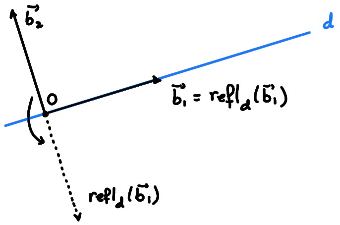
\[
\mathrm{refl}_d(\boldsymbol{b}_1)=\boldsymbol{b}_1\,\qquad
\mathrm{refl}_d(\boldsymbol{b}_2)=-\boldsymbol{b}_2\,.
\]
Par conséquent,
\[
[\mathrm{refl}_d]_{\mathcal{B}}=\bigl[[T(\boldsymbol{b}_1)]_\mathcal{B}\,[T(\boldsymbol{b}_2)]_\mathcal{B}\bigr]
=
\begin{pmatrix}
1&0\\
0&-1
\end{pmatrix}\,.
\]
À partir de cette expression simple, exprimons
la matrice de \(\mathrm{refl}_d\) relativement à une autre base, par exemple la base
canonique:
\[
[\mathrm{refl}_d]_{\mathcal{B}_{\mathrm{can}}}=
P_{\mathcal{B}_{\mathrm{can}}\mathcal{B}}
[\mathrm{refl}_d]_{\mathcal{B}}
P_{\mathcal{B}\mathcal{B}_{\mathrm{can}}}\,.
\]
Or
\[
[\boldsymbol{b}_1]_{\mathcal{B}_{\mathrm{can}}}= \begin{pmatrix} \cos \theta\\ \sin \theta \end{pmatrix}\,,\qquad
[\boldsymbol{b}_2]_{\mathcal{B}_{\mathrm{can}}}= \begin{pmatrix} -\sin\theta\\ \cos\theta \end{pmatrix}\,,
\]
et donc
\[
P_{\mathcal{B}_{\mathrm{can}}\mathcal{B}}=
\begin{pmatrix}
\cos \theta&-\sin\theta\\
\sin\theta&\cos\theta
\end{pmatrix}\,.
\]
Comme cette dernière est une matrice de rotation (d'un angle \(\theta\)), son
inverse est la matrice de rotation d'angle \(-\theta\). On a donc
\[\begin{aligned}
[\mathrm{refl}_d]_{\mathcal{B}_{\mathrm{can}}}&=
P_{\mathcal{B}_{\mathrm{can}}\mathcal{B}}
[\mathrm{refl}_d]_{\mathcal{B}}
P_{\mathcal{B}\mathcal{B}_{\mathrm{can}}}\\
&=
\begin{pmatrix}
\cos \theta&-\sin\theta\\
\sin\theta&\cos\theta
\end{pmatrix}
\begin{pmatrix}
1&0\\
0&-1
\end{pmatrix}
\begin{pmatrix}
\cos \theta&\sin\theta\\
-\sin\theta&\cos\theta
\end{pmatrix}\\
&=
\begin{pmatrix}
\cos^2\theta-\sin^2\theta&2\sin\theta\cos\theta\\
2\sin\theta\cos\theta&\sin^2\theta-\cos^2\theta
\end{pmatrix}\\
&=
\begin{pmatrix}
\cos(2\theta)&\sin(2\theta)\\
\sin(2\theta)&-\cos(2\theta)
\end{pmatrix}\,.
\end{aligned}\]
Cette expression est bien celle que nous avions obtenue précédemment.