Exemple: Considérons l'application linéaire \(T:\mathbb{R}^3\to\mathbb{R}^2\) définie par \[ T\left( \begin{pmatrix} x_1\\ x_2\\ x_3 \end{pmatrix} \right) := \begin{pmatrix} 2x_2-5x_3\\ x_1+3x_2 \end{pmatrix} = \begin{pmatrix} 0&2&-5\\ 1&3&0 \end{pmatrix} \begin{pmatrix} x_1\\ x_2\\ x_3 \end{pmatrix} \] Remarquons que lorsqu'une application est définie de cette façon, il est implicitement admis que les coordonnées (ici \(x_1,x_2,x_3\)) sont relativement aux bases canoniques des ensembles de départ et d'arrivée. Ici, pour les distinguer, nous noterons temporairement

• \({\color{magenta}\mathcal{B}_{\mathrm{can}}}=( {\color{magenta}\boldsymbol{e}_1}, {\color{magenta}\boldsymbol{e}_2}, {\color{magenta}\boldsymbol{e}_3})\) la base canonique de \(\mathbb{R}^3\),
• \({\color{blue}\mathcal{B}_{\mathrm{can}}}=( {\color{blue}\boldsymbol{e}_1}, {\color{blue}\boldsymbol{e}_2})\) la base canonique de \(\mathbb{R}^2\).

Donc la matrice ci-dessus est en fait \[\begin{aligned} [T]_{{\color{blue}\mathcal{B}_{\mathrm{can}}}{\color{magenta}\mathcal{B}_{\mathrm{can}}}} &= \bigl[ [T({\color{magenta}\boldsymbol{e}_1})]_{{\color{blue}\mathcal{B}_{\mathrm{can}}}} [T({\color{magenta}\boldsymbol{e}_2})]_{{\color{blue}\mathcal{B}_{\mathrm{can}}}} [T({\color{magenta}\boldsymbol{e}_3})]_{{\color{blue}\mathcal{B}_{\mathrm{can}}}} \bigr]\\ &= \begin{pmatrix} 0&2&-5\\ 1&3&0 \end{pmatrix} \end{aligned}\] Considérons maintenant les bases \(\mathcal{B}=(\boldsymbol{b}_1,\boldsymbol{b}_2,\boldsymbol{b}_3)\) de \(\mathbb{R}^3\) et \(\mathcal{C}=(\boldsymbol{c}_1,\boldsymbol{c}_2)\) de \(\mathbb{R}^2\), où \[ \boldsymbol{b}_1= \begin{pmatrix} 1\\ 1\\ 0 \end{pmatrix}\,,\quad \boldsymbol{b}_2= \begin{pmatrix} 1\\ 0\\ -1 \end{pmatrix}\,,\quad \boldsymbol{b}_3= \begin{pmatrix} 0\\ 1\\ 0 \end{pmatrix}\,,\quad \] \[ \boldsymbol{c}_1= \begin{pmatrix} 0\\ -1 \end{pmatrix}\,,\quad \boldsymbol{c}_2= \begin{pmatrix} 2\\ 3 \end{pmatrix}\,. \] Calculons la matrice de \(T\) relativement à ces deux nouvelles bases, \([T]_{\mathcal{B}\mathcal{C}}\). 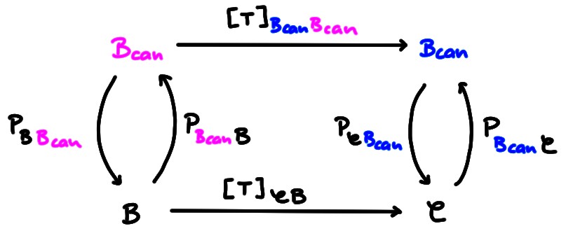On peut s'aider du schéma pour retrouver la formule: \[ [T]_{\mathcal{C}\mathcal{B}}= P_{\mathcal{C}{\color{blue}\mathcal{B}_{\mathrm{can}}}} [T]_{{\color{blue}\mathcal{B}_{\mathrm{can}}}{\color{magenta}\mathcal{B}_{\mathrm{can}}}} P_{{\color{magenta}\mathcal{B}_{\mathrm{can}}}\mathcal{B}} \] Or puisque les vecteurs de \(\mathcal{B}\) ont été donnés en composantes relativement à la base canonique, \[ [\boldsymbol{b}_1]_{\color{magenta}\mathcal{B}_{\mathrm{can}}}= \begin{pmatrix} 1\\ 1\\ 0 \end{pmatrix}\,,\quad [\boldsymbol{b}_2]_{\color{magenta}\mathcal{B}_{\mathrm{can}}}= \begin{pmatrix} 1\\ 0\\ -1 \end{pmatrix}\,,\quad [\boldsymbol{b}_3]_{\color{magenta}\mathcal{B}_{\mathrm{can}}}= \begin{pmatrix} 0\\ 1\\ 0 \end{pmatrix}\,,\quad \] on a déjà \[ P_{{\color{magenta}\mathcal{B}_{\mathrm{can}}}\mathcal{B}} = \bigl[ [\boldsymbol{b}_1]_{\color{magenta}\mathcal{B}_{\mathrm{can}}}\, [\boldsymbol{b}_2]_{\color{magenta}\mathcal{B}_{\mathrm{can}}}\, [\boldsymbol{b}_3]_{\color{magenta}\mathcal{B}_{\mathrm{can}}} \bigr] = \begin{pmatrix} 1&1&0\\ 1&0&1\\ 0&-1&0 \end{pmatrix}\,. \] Ensuite, \[ [\boldsymbol{c}_1]_{\color{blue}\mathcal{B}_{\mathrm{can}}}= \begin{pmatrix} 0\\ -1 \end{pmatrix}\,,\quad [\boldsymbol{c}_2]_{\color{blue}\mathcal{B}_{\mathrm{can}}}= \begin{pmatrix} 2\\ 3 \end{pmatrix}\,, \] et donc \[\begin{aligned} P_{\mathcal{C}{\color{blue}\mathcal{B}_{\mathrm{can}}}} &= {P_{{\color{blue}\mathcal{B}_{\mathrm{can}}}\mathcal{C}}}^{-1}\\ &=\bigl[[\boldsymbol{c}_1]_{\color{blue}\mathcal{B}_{\mathrm{can}}}\, [\boldsymbol{c}_2]_{\color{blue}\mathcal{B}_{\mathrm{can}}}\bigr]^{-1}\\ &= \begin{pmatrix} 0&2\\ -1&3 \end{pmatrix}^{-1} = \begin{pmatrix} 3/2&-1\\ 1/2&0 \end{pmatrix} \end{aligned}\] On a donc \[\begin{aligned} [T]_{\mathcal{C}\mathcal{B}}&= P_{\mathcal{C}{\color{blue}\mathcal{B}_{\mathrm{can}}}} [T]_{{\color{blue}\mathcal{B}_{\mathrm{can}}}{\color{magenta}\mathcal{B}_{\mathrm{can}}}} P_{{\color{magenta}\mathcal{B}_{\mathrm{can}}}\mathcal{B}}\\ &= \begin{pmatrix} 3/2&-1\\ 1/2&0 \end{pmatrix} \begin{pmatrix} 0&2&-5\\ 1&3&0 \end{pmatrix} \begin{pmatrix} 1&1&0\\ 1&0&1\\ 0&-1&0 \end{pmatrix}\\ &= \begin{pmatrix} -1&13/2&0\\ 1&5/2&1 \end{pmatrix} \end{aligned}\]

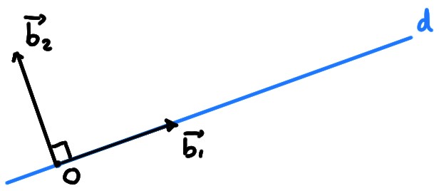
Exemple: Considérons la projection \(\mathrm{proj}_d\) sur une droite \(d\) passant par l'origine et faisant un angle de \(\theta\) avec \(\boldsymbol{e}_1\):

Rappelons que sa matrice relativement à la base canonique est donnée par \[ [\mathrm{proj}_d]_{\mathcal{B}_{can}} = \begin{pmatrix} \cos^2\theta&\cos\theta\sin\theta\\ \cos\theta\sin\theta&\sin^2\theta \end{pmatrix} \] Plus naturelle, pour décrire cette projection, serait une base dans laquelle les vecteurs sont orientés dans des directions qui tiennent compte de la position de l'axe \(d\). Par exemple, une base \(\mathcal{B}=(\boldsymbol{b}_1,\boldsymbol{b}_2)\) où \(\boldsymbol{b}_1\) dirige \(d\), et \(\boldsymbol{b}_2\) est perpendiculaire à \(d\): Par définition de la projection, \[ \mathrm{proj}_d(\boldsymbol{b}_1)=\boldsymbol{b}_1\,,\qquad \mathrm{proj}_d(\boldsymbol{b}_2)=\boldsymbol{0}\,, \] ce qui donne \[ [\mathrm{proj}_d(\boldsymbol{b}_1)]_{\mathcal{B}}= \begin{pmatrix} 1\\ 0 \end{pmatrix} \,,\qquad [\mathrm{proj}_d(\boldsymbol{b}_2)]_{\mathcal{B}}= \begin{pmatrix} 0\\ 0 \end{pmatrix}\,. \] Par conséquent, la matrice relativement à cette base prend une forme particulièrement simple: \[ [\mathrm{proj}_d]_{\mathcal{B}}= \begin{pmatrix} 1&0\\ 0&0 \end{pmatrix} \] Vérifions que c'est bien ce que l'on obtient en faisant le changement de base, de \(\mathcal{B}_{\mathrm{can}}\) vers \(\mathcal{B}\).

Tout d'abord, on écrit explicitement les vecteurs de la nouvelle base en fonction de ceux de l'ancienne. Puisque \(d\) fait un angle \(\theta\) avec l'horizontale, en les prenant orientés comme sur la figure ci-dessus, et unitaires, \[ [\boldsymbol{b}_1]_{\mathcal{B}_{\mathrm{can}}}= \begin{pmatrix} \cos\theta\\ \sin\theta \end{pmatrix}\,,\qquad [\boldsymbol{b}_2]_{\mathcal{B}_{\mathrm{can}}}= \begin{pmatrix} -\sin\theta\\ \cos\theta \end{pmatrix}\,. \] Ainsi, la matrice de changement de base est \[ P_{\mathcal{B}_{\mathrm{can}}\mathcal{B}}= \begin{pmatrix} \cos\theta&-\sin\theta \\ \sin\theta & \cos\theta \end{pmatrix}\,. \] La formule du changement de base donne donc \[\begin{aligned} [\mathrm{proj}_d]_{\mathcal{B}} &= {P_{\mathcal{B}_{\mathrm{can}}\mathcal{B}}}^{-1} [\mathrm{proj}_d]_{\mathcal{B}_{\mathrm{can}}} P_{\mathcal{B}_{\mathrm{can}}\mathcal{B}}\\ =& \begin{pmatrix} \cos\theta&\sin\theta \\ -\sin\theta & \cos\theta \end{pmatrix} \begin{pmatrix} \cos^2\theta&\cos\theta\sin\theta\\ \cos\theta\sin\theta&\sin^2\theta \end{pmatrix} \begin{pmatrix} \cos\theta&-\sin\theta \\ \sin\theta & \cos\theta \end{pmatrix}\\ =& \begin{pmatrix} 1&0\\ 0&0 \end{pmatrix}\,. \end{aligned}\]

Exemple: Considérons la réflexion par rapport à une droite \(d\) qui passe par l'origine, que nous avions notée \(\mathrm{refl}_d\). Utilisons à nouveau la base \(\mathcal{B}=(\boldsymbol{b}_1,\boldsymbol{b}_2)\) du dernier exemple, où \(\boldsymbol{b}_1\) dirige \(d\), et \(\boldsymbol{b}_2\) est perpendiculaire à \(d\). On remarque que l'application de la réflexion sur ces vecteurs prend une forme très simple:

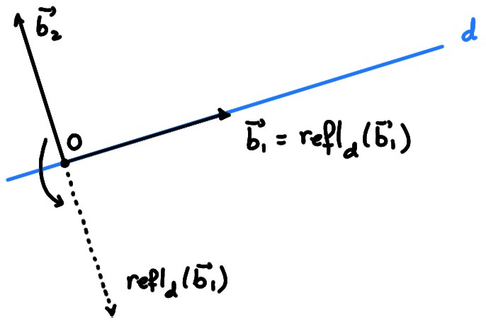
\[ \mathrm{refl}_d(\boldsymbol{b}_1)=\boldsymbol{b}_1\,\qquad \mathrm{refl}_d(\boldsymbol{b}_2)=-\boldsymbol{b}_2\,. \] Par conséquent, \[ [\mathrm{refl}_d]_{\mathcal{B}}=\bigl[[\mathrm{refl}_d(\boldsymbol{b}_1)]_\mathcal{B}\, [\mathrm{refl}_d(\boldsymbol{b}_2)]_\mathcal{B}\bigr] = \begin{pmatrix} 1&0\\ 0&-1 \end{pmatrix}\,. \] Maintenant, exprimons la matrice de \(\mathrm{refl}_d\) relativement à la base canonique: Puisque la matrice de changement de base est la même qu'avant, \[\begin{aligned} [\mathrm{refl}_d]_{\mathcal{B}_{\mathrm{can}}}&= P_{\mathcal{B}_{\mathrm{can}}\mathcal{B}} [\mathrm{refl}_d]_{\mathcal{B}} P_{\mathcal{B}_{\mathrm{can}}\mathcal{B}}^{-1}\\ &= \begin{pmatrix} \cos \theta&-\sin\theta\\ \sin\theta&\cos\theta \end{pmatrix} \begin{pmatrix} 1&0\\ 0&-1 \end{pmatrix} \begin{pmatrix} \cos \theta&\sin\theta\\ -\sin\theta&\cos\theta \end{pmatrix}\\ &= \begin{pmatrix} \cos^2\theta-\sin^2\theta&2\sin\theta\cos\theta\\ 2\sin\theta\cos\theta&\sin^2\theta-\cos^2\theta \end{pmatrix}\\ &= \begin{pmatrix} \cos(2\theta)&\sin(2\theta)\\ \sin(2\theta)&-\cos(2\theta) \end{pmatrix}\,. \end{aligned}\] Cette expression est bien celle que nous avions obtenue précédemment.